Welcome
- To deploy the app on command line or to create a URL using Heroku, access our GitHub repository here
About
These tools aim to provide a reproducible and consistent data visualisation platform where experimental and computational researchers can use random forest and statistical analysis to find the best materials for specific applications. Random forest is a supervised machine learning model that can be used to perform regression tasks. The model learns to map data (features or descriptors) by constructing a multitude of decision trees to an output (target variable) in the training phase of the model. Hyperparameter tuning is also used to optimise and tune the algorithm. It uses bagging and feature randomness when building each individual tree to try to create an uncorrelated forest of trees that predicts the target variable more accurately than a single decision tree.
Data File Requirements
The data file to upload must meet the following requirements:
1. A .xlsx, .csv or a .txt data file must be uploaded. Please note that large .xlsx files take time to process so .csv or .txt files are preferred. For .txt files the application only accepts comma text separators.
2. The uploaded datasheet must have the structure name or identifier on its first column (shown in table 1).
3. The uploaded datasheet must be completely populated (no blank cells). Blank cells can be replaced to ‘0’ using the ‘Replace All’ function in Excel. No symbols should be used in the spreadsheet.
4. Data must be tidy data. If required, data must be transposed so that there is a single column stating the variables simulated with a column for the desired animation frame containing discrete numerical values (e.g. pressures). Example data files before e.g. AAML_Oxygen_Raw_Data.csv and after transposition AAML_Oxygen_Data.csv can be found here
Table 1: Example File Upload
| DDEC code | Family | Pressure | Grav. Uptake (mol/kg) | Vol. Uptake (cm3/cm3) | Qst (kJ/mol) | … |
|---|---|---|---|---|---|---|
| AFIXAO | ZIF | 1 | 0.3379 | 8.4985 | 15.6505 | … |
| ABUWOJ | ZnO | 1 | 0.5687 | 14.7654 | 16.5644 | … |
| AVAQIX | None | 1 | 0.8956 | 26.2387 | 18.2041 | … |
| HOWPUF | None | 1 | 0.3486 | 7.5929 | 19.7446 | … |
| HOWQAM | None | 5 | 0.5020 | 11.4214 | 15.7436 | … |
| HOWQEQ | None | 5 | 0 | 17.5332 | 16.8026 | … |
| HOXKUB | None | 5 | 0.4167 | 16.0261 | 20.7236 | … |
| … | … | … | … | … | … | … |
The tab of the app will fade when the app is computing a user input. It will return to its original color once it has completed the user's input (Figure 2). In addition to the faded tab, the dashboard browser tab will show “Updating…” when the tool is updating the data. Wait for this to return to ‘Dash’ before using the tool. This is when the file upload is complete.
Functions found on 2D Plots
Download plots
As shown in the picture, click on the camera icon and get the plot in PNG format.
![]()
Pan mode
If the plot’s drag mode is set to ‘Pan’, click and drag on the plot to pan and double-click to reset the pan.
![]()
Zoom modes
If the plot’s mode is set to ‘Zoom’, click and drag on the plot to zoom-in and double click to zoom-out completely. i.e. auto scale of both axis. The user can also zoom in and out by clicking on the + and – buttons. Axes labels will automatically optimize as you zoom in.
![]()
Reset axes
One can also drag the x and y axis in a horizontal and vertical motion respectively to move along the length of the axis. When the user drags the middle of the axis, a double headed arrow will appear. This allows the user to adjust the range of the axis i.e. both the lower and upper bound (Figure 6). Clicking ‘Reset axes’ will reset the axes.
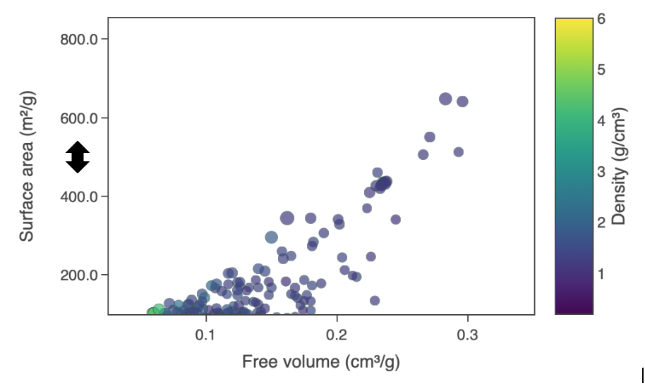
Figure 6: Reset axis double headed arrow
When the user drags the top of the axis or the bottom of the axis, a single headed arrow will appear. This allows the user to adjust only the upper limit of the axis i.e. the upper bound or the lower limit of the axis i.e. the lower bound respectively. (Figure 7). Clicking 'Reset axes' will reset the axes.
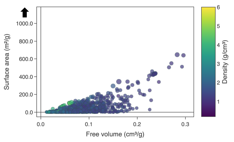
Figure 7: Reset axis single headed arrow
Hover options
One of these two buttons is selected at all times. Clicking ‘Show closest data on hover’ will display the data for just one point under the cursor. Clicking ‘Compare data on hover’ will show you the data for all points with the same x-value.

Preparing Data for RF
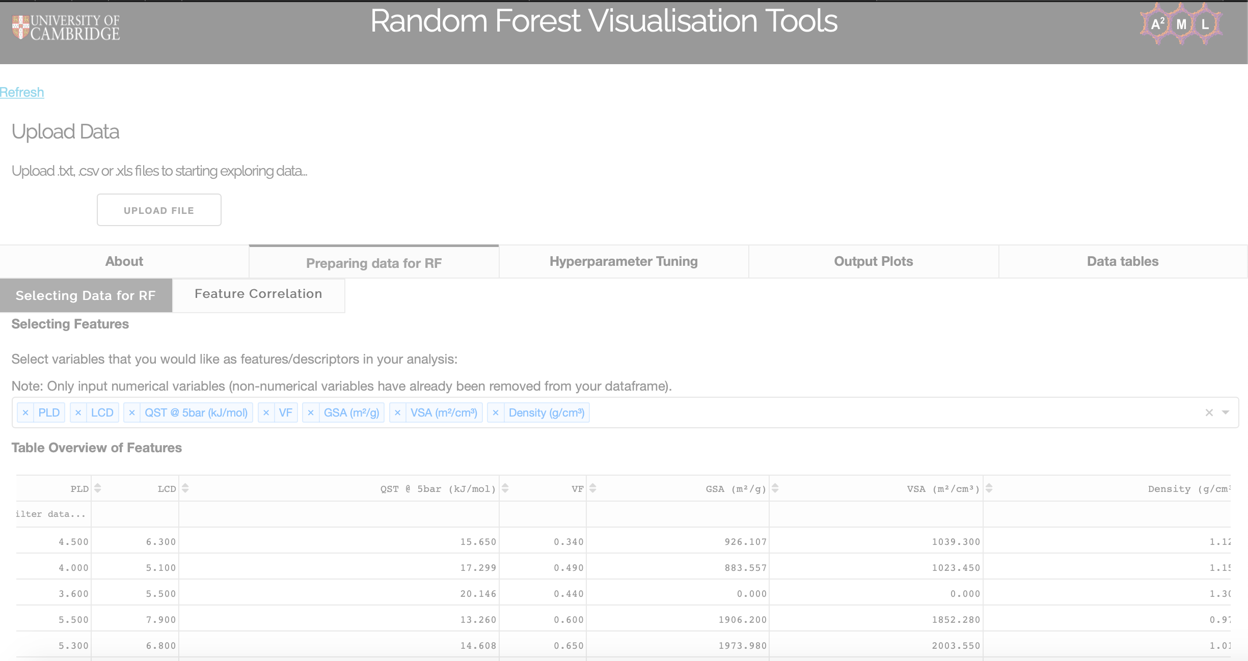
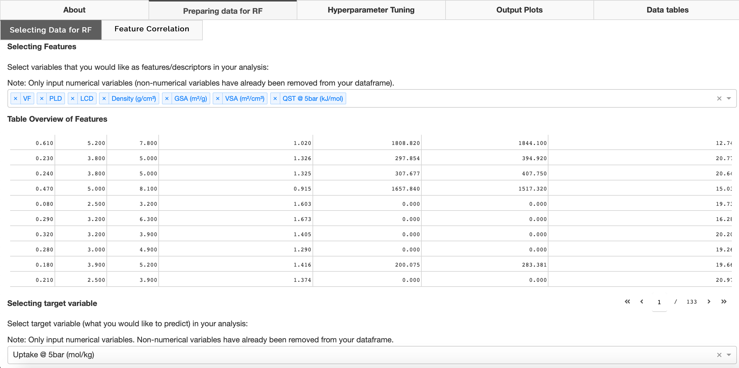
Selecting data for RF
Users can select which variables they would like as features and select their target variable in the 'Selecting Data for RF' tab. Non-numerical values are removed from the user's data frame and a table of selected features is populated.
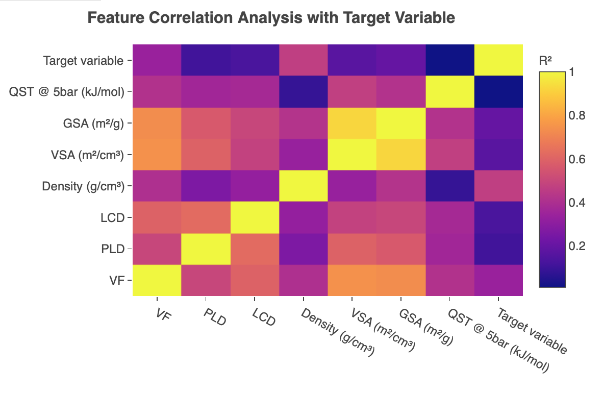
Feature correlation
In the 'Feature Correlation' tab, a heatmap of the coefficient of determination of features and the target variable is also produced, allowing users to see correlations between the variables used.
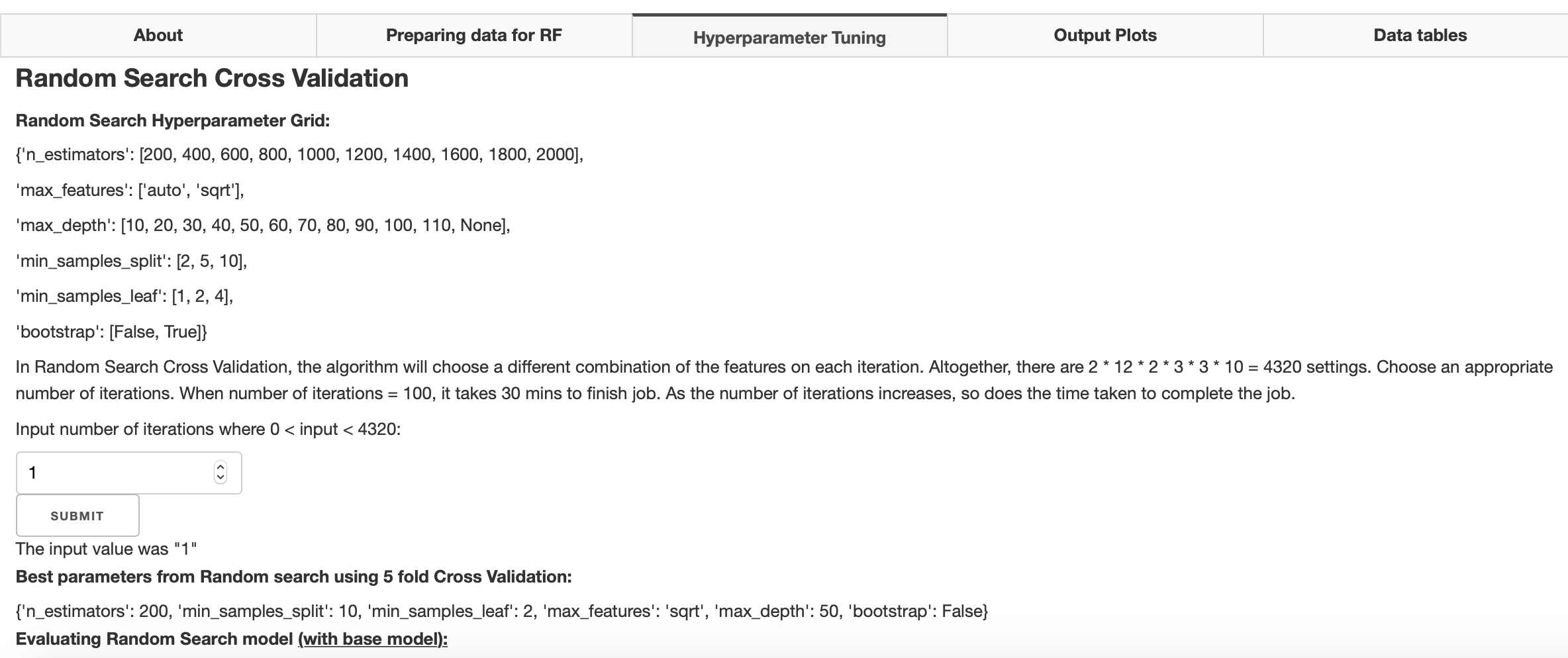
Hyperparameter tuning
Hyperparameter tuning is a way one can optimise their random forest model by changing settings in their algorithm to optimise its performance. These hyperparameters are set before training the model. Scikit-learn uses a set of default hyperparameters for all models but these may not be optimal. In the apps hyperparameter tuning, 5-Fold Cross- Validation is used to obtain optimal hyperparameters from a random hyperparameter grid. Random search will randomly test n number of iterations, where n is a number inputted by the user, to find the best hyperparameters. These hyperparameters are then used to create a second grid search where all possible hyperparameter settings in this grid are tested. The optimal hyperparameters from this grid search are then used as hyperparameters in the user's random forest model. This part of the tool requires the most time. When computing, the apps background will become faded and a loading cursor will appear. The process of your hyperparameter tuning can be trailed on the terminal as the user runs the app.
Once completed, optimal hyperparameters with improvement in accuracy compared to the base model (default hyperparameters) will be computed. These hyperparameters will automatically be used in the final random forest model.
Output plots
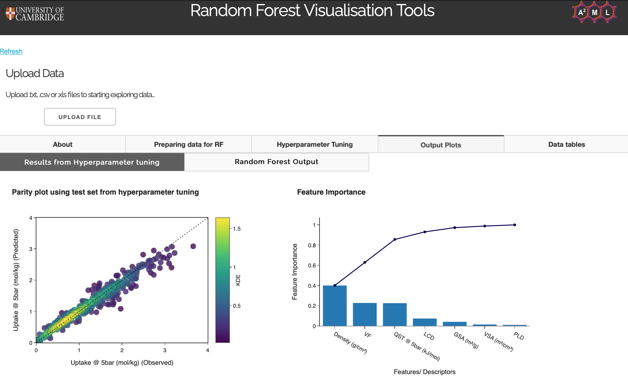
Once the app has computed the optimal hyperparameters, a parity plot using these hyperparameters will appear in the Results from 'Hyperparameter tuning' tab. A bar plot of feature importance and cumulative feature importance will also appear. This is not the final output of the model but useful to look at to analyse model performance metrics, overfitting, and feature engineering.
Results from Hyperparameter tuning
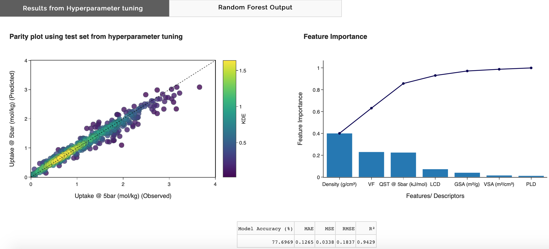
Figure 10: Results from Hyperparameter tuning tab
Random Forest Output
In the 'Random Forest Output' tab, the user can determine a new test size to compute the final random forest result. This will take a few seconds to compute. A feature importance bar plot will also appear which can be useful to see which features were considered most important in the model and which features can be removed to improve run time. In the subtab 'Error Plots', an error distribution of the models observed and predicted values is available as well as a scatter plot illustrating model error in percentage terms and observed values.
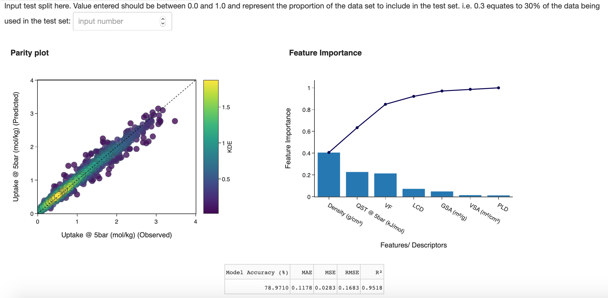
Figure 11: Random Forest Output
Error Plot
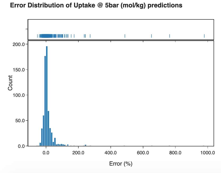
Figure 12: Error plot distribution

Figure 13: Error and observed values scatter plot
Data tables
The user's inputs across the app will provide the output of the data tables. The user can download the feature and target variable correlations, performance metrics, random forest data and feature importance data from the 'Random Forest Output' tab.
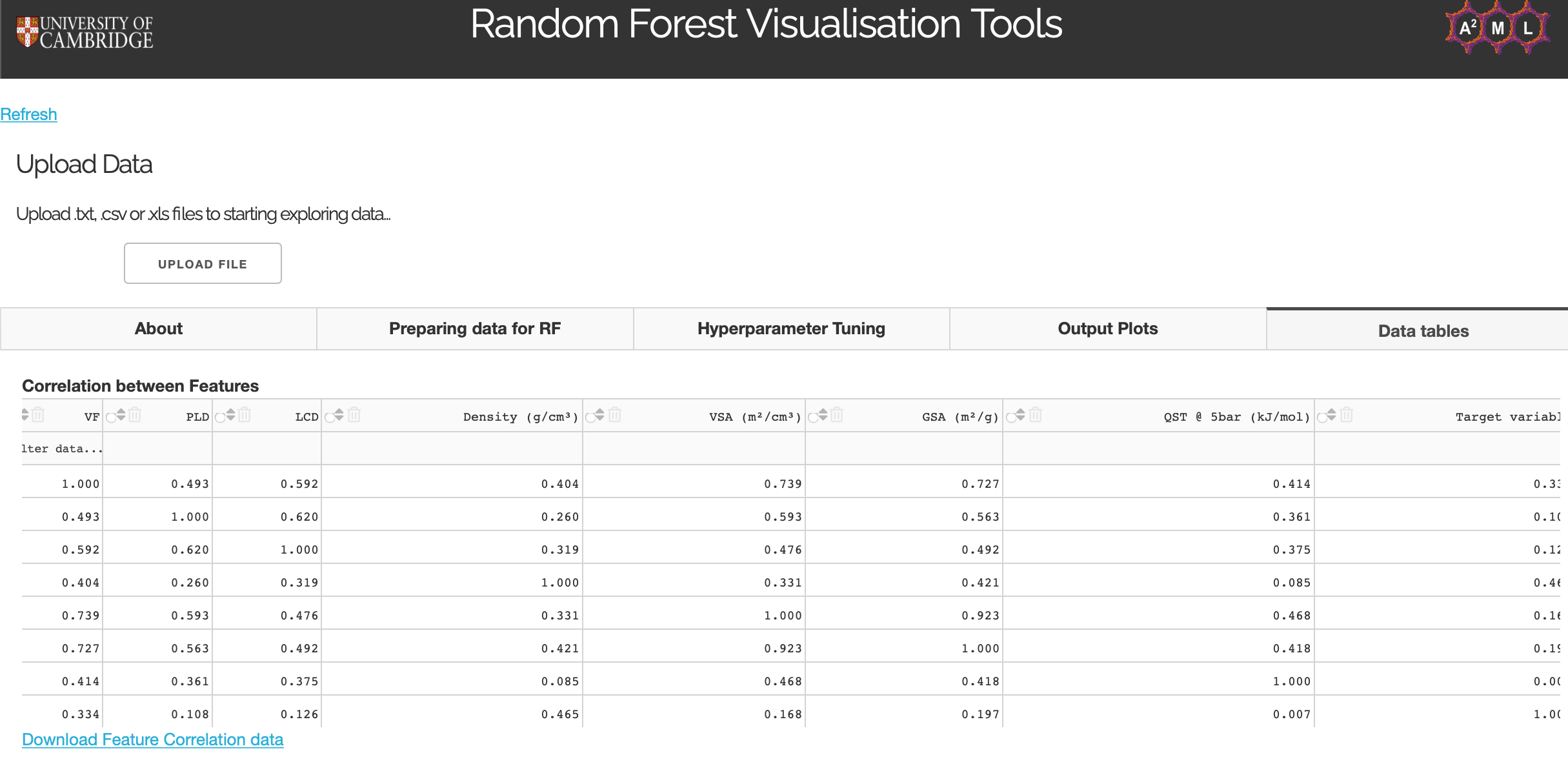
Figure 14: Downloadable data tables
Contributing
For changes, please open an issue first to discuss what you would like to change. You can also contact the AAML research group to discuss further contributions and collaborations.
Contact Us
![]()
Email:
Mythili Sutharson,
Nakul Rampal,
Rocio Bueno Perez,
David Fairen Jimenez
Website: http://aam.ceb.cam.ac.uk/
Address:
Cambridge University,
Philippa Fawcett Dr,
Cambridge
CB3 0AS
License
This project is licensed under the MIT License - see the LICENSE.md file for details
Acknowledgments
- AAML Research Group for developing this dashboard for the MOF community. Click here to read more about our work
- Dash - the python framework used to build this web application